Local Search

Local Search differs from other algorithms such as depth first and A* search. We use Local Search when we are interested only in the goal state and the path is irrelevant. It is useful when the state space is too large, the evaluation function is computationally expensive or when optimality is not required.

How Local Search works

Local Search works by incrementally improve the current best state by exploring neighbouring states with higher utility. It does not keep track of previous states, so it is memory efficient.

Hill climbing search

Local Search can solve an optimisation problem by finding the best state according to an objective function. The optimisation starts with a random initial state. The agent then observes the local neighbourhood around this state. The state then changes to one with a higher utility. This process repeats until a local optimum is reached.

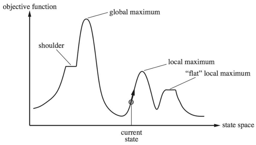
This process works very quickly to improve from a bad initial state, however it is often not optimal. This is because the objective function is likely to be non-convex. This will cause the process to possibly end on a local maxima, rather than a global maxima. One must also be aware of ridges (sequence of local maxima) and plateaus (areas of constant utility), which may make the agent fail to terminate (i.e. not complete). The algorithm is also greedy - It does not look beyond the small neighbourhood.

Figure 1- An Example Optimisation Problem

How to improve Local Search

In order to overcome the limitations of local search as stated above, there are various modifications one can make to the implementation.

Hill Climbing with sideways move

If the agent is at a local maxima, the agent will be able to move sideways along the local maxima, as long as the utility does not decrease (i.e. a shoulder or a plateau). This will help if the local maxima is a shoulder, however a plateau will cause the agent to wander aimlessly - so a limit on sideways moves must be set.

Hill Climbing with random restarts

Having a series of hill climbing searches with randomly generated initial states. The highest utility value of these searches is likely the global maxima, and thus the optimal solution. However, this process may be inefficient especially for multi-dimensional problems.

Simulated Annealing

With simulated annealing, the agent is allowed to occasionally make "bad" moves that lower utility. A temperature parameter T is also introduced. At high temperatures, the likelihood of the agent making a bad move is high, while there is a low likelihood when the temperature is low. Over time, the temperature decreases. A global optimal will be reached if the cooling rate is slow enough, however this may not be possible.

Beam Search

Beam search uses multiple states which can communicate with each other to decide their next successors. The "Beam" in Beam Search refers to the number of states maintained.

How it works

Initialise K randomly generated states. For each state k find the successor state j. Then sort to find the best K states. Repeat the process with these states until they converge at a local maxima.

Beam search can work quickly, however it may suffer from a lack of diversity, a variant known as stochastic beam search fixes the problem. (Note to self: figure out wtf this means)

Blog post on beam search in language translation

Genetic Algorithm

Variant of stochastic beam search that generates successors from pairs of states. It is inspired by natural selection.

How it works

First a set of randomly generated states are initialised. Each individual state is encoded into binary. This is its gene representation. This is done by mapping the objective function f(x) with a domain of [x_min,x_max] to [0,2^q-1] where q is the number of binary digits. Each x value is mapped to its corresponding binary using this formula:
x = x_min + ((x_max - x_min)/2^q - 1) × ∑(b_q × 2^{m - 1}) for 1 ≤ m ≤ q.
The larger q is, the more values of x can be mapped within the domain.

Then a fitness evaluation occurs on each individual state. States that have a fitness below a certain threshold may be culled or they may be less likely to reproduce.

States that can reproduce may then perform crossover with their partner. This is when a random section of the genetic code is swapped with the partner (as in crossover with chromosomes).

There is also a random chance for mutation to occur, where a single bit in the gene is flipped.

The simulation ends after a fixed number of generations (normally 100), or if the execution has taken too long, or if the standard deviation of the fitness' drops too much, or if fitness no longer improves.

The genetic algorithm does not guarantee a global optimal, however it is easy to parallelise and implement. However, its success is dependent on a good fitness function and initial conditions (population size, mutation rate etc.)